import IPython.display as ipd
from IPython.display import Image
from IPython.display import Audio
import numpy as np
import pandas as pd
import scipy
import matplotlib.pyplot as plt
from collections import OrderedDict
import librosa
import librosa.display
from utils.plot_tools import plot_signal, plot_matrix
# from util import *2.3. 오디오 표현
Audio Representation
음악표현
화성
스펙트로그램
음악의 표현 방법 중 오디오 표현에 대해 알아본다. 음파(wave), 주파수(frequency), 고조파(harmonics), 강도(intensity), 라우드니스(loudness), 음색(timbre) 등의 중요한 개념을 포함한다.
이 글은 FMP(Fundamentals of Music Processing) Notebooks을 참고로 합니다.
오디오 표현 (Audio Representation)
- 음파(waveform)
- 피치(pitch)와 주파수(frequency)
- 고조파(harmonics)
- 다이내믹(dynamics), 강도(intensity), 라우드니스(loudness)
- 음색(timbre)
- 음악가들은 악보를 연주할 때 소리를 기압 진동을 통해 공기로 보낸다. 간단히 말해 소리는 공기 진동이다. 소리는 종파(longitundinal waves)를 통해 진동한다.
- 오디오는 인간이 들을 수 있는 소리의 생산, 전송 또는 수신을 의미한다.
- 오디오 신호는 진동에 의해 발생하는 기압의 변동을 시간의 함수로 나타내는 소리의 표현이다.
- 악보나 기호 표현과는 달리, 오디오 표현은 음악의 음향적 실현을 재현하는 데 필요한 모든 것을 인코딩한다. 그러나 온셋(onset), 지속 시간(duration) 및 피치와 같은 참고 매개 변수는 명시적으로 인코딩되지 않는다.
음파 (Waveforms)
- 소리는 가수의 성대, 바이올린의 현과 소리판 등의 진동하는 물체에 의해 발생한다. 이러한 진동은 공기 분자의 변위와 진동을 유발하여 지역적인 압축(compression)과 희박화(rarefaction)를 초래한다.
- 교류 압력(alternating pressure)은 공기를 통해 파동으로 청취자 또는 마이크로 전달된다. 이는 사람에 의해 소리로 인식되거나 마이크에 의해 전기 신호로 변환될 수 있다.
- 특정 위치의 기압 변화는 pressure-time plot으로 나타낼 수 있으며, 이는 파형(waveform)이라고도 한다.
Image("../img/2.music_representation/FMP_C1_F17.png", width=500)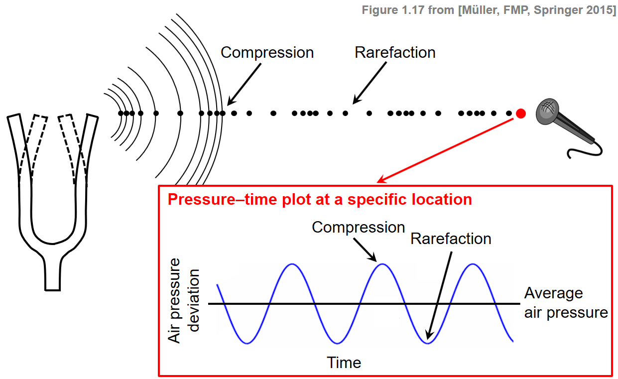
x, sr = librosa.load('../audio/c_strum.wav')
print("샘플링 레이트: ",sr)
ipd.Audio(x, rate=sr)샘플링 레이트: 22050- 위 오디오를 파형으로 보이면 다음과 같다.
plot_signal(x,sr,ylabel='Amplitude')
plt.show()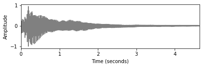
- 공기압이 높은 지점과 낮은 지점이 번갈아가며 규칙적으로 반복되는 경우, 파형이 주기적(periodic)이라고 한다.
- 이 경우 파동의 주기는 주기를 완료하는 데 필요한 시간으로 정의된다.
- 헤르츠(Hz) 단위로 측정된 주파수는 이러한 주기의 역수이다.
- 다음 그림은 가장 단순한 유형의 주기 파형인 정현파(sinusoid)를 보여준다.
- 이 예에서 파형의 주기는 25초이므로 주파수는 4Hz이다.
- 주기적 파형의 가장 단순한 유형은 정현파이며, 주파수(frequency), 진폭(amplitude)(평균에서 사인파의 피크 편차), 위상(phase)(주기에서 정현파가 0인 위치를 결정함)에 의해 완전하게 지정된다.
Image("../img/2.music_representation/FMP_C1_F19.png", width=600)
Fs = 100
duration = 2
amplitude = 1.5
phase = 0.1
frequency = 3
num_samples = int(Fs * duration)
t = np.arange(num_samples) / Fs
x = amplitude * np.sin(2 * np.pi * (frequency * t - phase))
plt.figure(figsize=(6, 2))
plt.plot(t, x, linewidth=2.0)
plt.xlim([0, duration])
plt.xlabel('Time (seconds)')
plt.ylabel('Amplitude')
plt.tight_layout()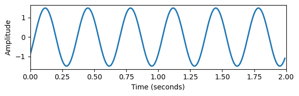
- 디지털 컴퓨터는 이 데이터를 이산(discrete) 시간으로 밖에 포착하지 못한다.
- 컴퓨터가 잡는 오디오 데이터의 속도/레이트(rate)를 샘플링 주파수, 샘플링 레이트(sampling frequency, sampling rate)라고 한다.
- 예를 들어 샘플링 레이트가 44100 Hz이면 보통 CD 레코딩의 샘플링 레이트이다. https://en.wikipedia.org/wiki/Sampling_(signal_processing)#Audio_sampling
주파수와 피치 (Frequency and Pitch)
- 주파수 설명 참고 (한글): http://www.ktword.co.kr/test/view/view.php?m_temp1=4148
들을 수 있는 주파수 범위
정현파(sinusoidal wave)의 주파수가 높을수록 더 높은 소리를 낸다.
인간의 가청 주파수 범위는 약 20Hz와 20000Hz(20 kHz) 사이이다. 다른 동물들은 다른 청력 범위를 가지고 있다. 예를 들어, 개의 청력 범위의 상단은 약 45kHz이고 고양이의 청력은 64kHz인 반면, 박쥐는 심지어 100kHz 이상의 주파수를 감지할 수 있다. 이는 사람의 청각 능력을 뛰어넘는 초음파를 내는 개 호루라기를 이용해 주변 사람들을 방해하지 않고 동물을 훈련시키고 명령할 수 있는 이유이다.
다음 실험에서 주파수가 초당 2배(1옥타브) 증가하는 처프(chirp) 신호를 생성한다.
def generate_chirp_exp_octave(freq_start=440, dur=8, Fs=44100, amp=1):
"""Generate one octave of a chirp with exponential frequency increase
Args:
freq_start (float): Start frequency of chirp (Default value = 440)
dur (float): Duration (in seconds) (Default value = 8)
Fs (scalar): Sampling rate (Default value = 44100)
amp (float): Amplitude of generated signal (Default value = 1)
Returns:
x (np.ndarray): Chirp signal
t (np.ndarray): Time axis (in seconds)
"""
N = int(dur * Fs)
t = np.arange(N) / Fs
x = np.sin(2 * np.pi * freq_start * np.power(2, t / dur) / np.log(2) * dur)
x = amp * x / np.max(x)
return x, t# 20Hz부터 시작하여 주파수는 총 10초 동안 20480Hz까지 상승한다.
Fs = 44100
dur = 1
freq_start = 20 * 2**np.arange(10)
for f in freq_start:
if f==freq_start[0]:
chirp, t = generate_chirp_exp_octave(freq_start=f, dur=dur, Fs=Fs, amp=.25)
else:
chirp_oct, t = generate_chirp_exp_octave(freq_start=f, dur=dur, Fs=Fs, amp=.25)
chirp = np.concatenate((chirp, chirp_oct))
ipd.display(ipd.Audio(chirp, rate=Fs))# 640Hz부터 시작하여 주파수는 총 10초 동안 20Hz까지 하락한다.
Fs = 8000
dur = 2
freq_start = 20 * 2**np.arange(5)
for f in freq_start:
if f==freq_start[0]:
chirp, t = generate_chirp_exp_octave(freq_start=f, dur=dur, Fs=Fs, amp=1)
else:
chirp_oct, t = generate_chirp_exp_octave(freq_start=f, dur=dur, Fs=Fs, amp=1)
chirp = np.concatenate((chirp,chirp_oct))
chirp = chirp[::-1]
ipd.display(ipd.Audio(chirp, rate=Fs))피치와 중심 주파수(center frequency)
정현파는 음의 음향적 실현의 원형으로 간주될 수 있다. 때때로 정현파에서 나오는 소리를 하모닉 사운드(harmonic sound) 또는 순수 음색(pure tone)이라고 한다.
주파수의 개념은 소리의 피치를 결정하는 것과 밀접한 관련이 있다. 일반적으로 피치는 소리의 주관적인 속성이다.
복잡한 혼합음의 경우, 주파수와의 관계가 특히 모호할 수 있다. 그러나 순수 음색의 경우 주파수와 피치의 관계가 명확하다. 예를 들어, 440 Hz의 주파수를 갖는 정현파는 피치 A4에 해당한다. 이 특정한 피치는 콘서트 피치(concert pitch)로 알려져 있으며, 이는 연주를 위해 악기가 튜닝되는 기준 피치로 사용된다.
주파수의 약간의 변화가 반드시 지각할 수 있는 변화로 이어지는 것은 아니기 때문에, 일반적으로 주파수의 전체 범위를 단일 피치와 연관시킨다.
두 주파수가 2의 거듭제곱에 의해 차이가 나는 경우, 이는 옥타브의 개념과 연관된다.
- 예를 들어, 피치 A3(220 Hz)와 피치 A4(440 Hz) 사이의 인식 거리는 피치 A4와 피치 A5(880 Hz) 사이의 인식 거리와 동일하다.
- 즉, 피치에 대한 인간의 인식은 본질적으로 로그(logarithm)이다. 이 지각 특성은 이미 로그 주파수 축을 기준으로 옥타브를 12개의 반음으로 세분화하는 평균율(“equal-tempered scale”)을 정의하는 데 사용되었다.
더 공식적으로, MIDI 노트 번호를 사용하여, 다음과 같이 정의된 중심 주파수(center frequency) \(F_{pitch}(p)\)(Hz 단위로 측정)를 각 피치 \(p∈[0:127]\) 에 연결할 수 있다.
- \(F_{pitch}(p)=2^{(p−69)/12} \cdot 440\)
- MIDI 노트 번호 \(p=69\)는 기준으로 사용되며 피치 A4(440Hz)에 해당된다. 피치 넘버를 12(옥타브) 증가시키면 2배 증가한다. \(F_{pitch} ( p + 12) = 2 \cdot F_{pitch} ( p)\)
- \(F_{pitch}(p)=2^{(p−69)/12} \cdot 440\)
Image("../img/2.music_representation/FMP_C1_MIDI-NoteNumbers.png", width=500)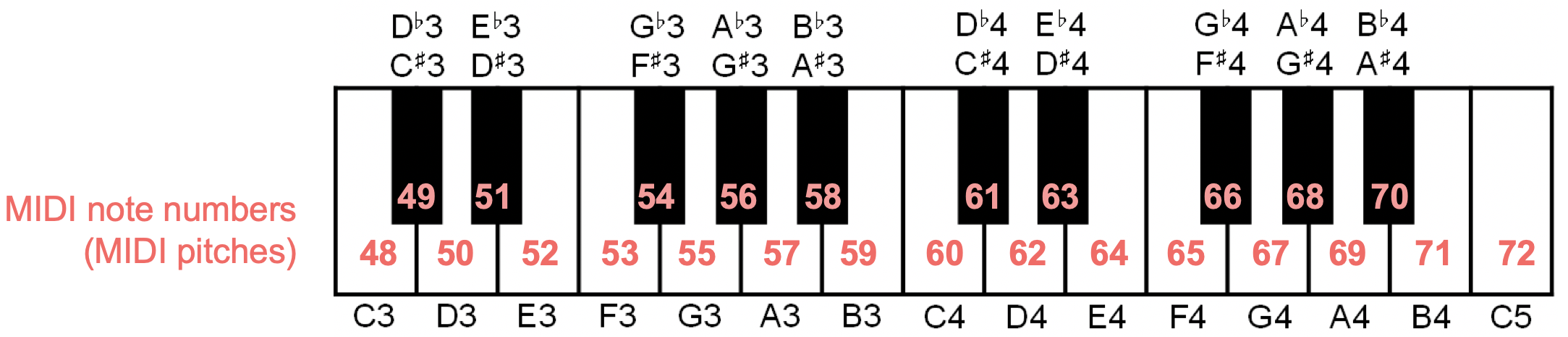
def f_pitch(p):
"""Compute center frequency for (single or array of) MIDI note numbers
Args:
p (float or np.ndarray): MIDI note numbers
Returns:
freq_center (float or np.ndarray): Center frequency
"""
freq_center = 2 ** ((p - 69) / 12) * 440
return freq_center
chroma = ['A ', 'A#', 'B ', 'C ', 'C#', 'D ', 'D#', 'E ', 'F ', 'F#', 'G ', 'G#']
for p in range(21, 109):
print('p = %3d (%2s%1d), freq = %7.2f ' % (p, chroma[(p-69) % 12], (p//12-1), f_pitch(p)))p = 21 (A 0), freq = 27.50
p = 22 (A#0), freq = 29.14
p = 23 (B 0), freq = 30.87
p = 24 (C 1), freq = 32.70
p = 25 (C#1), freq = 34.65
p = 26 (D 1), freq = 36.71
p = 27 (D#1), freq = 38.89
p = 28 (E 1), freq = 41.20
p = 29 (F 1), freq = 43.65
p = 30 (F#1), freq = 46.25
p = 31 (G 1), freq = 49.00
p = 32 (G#1), freq = 51.91
p = 33 (A 1), freq = 55.00
p = 34 (A#1), freq = 58.27
p = 35 (B 1), freq = 61.74
p = 36 (C 2), freq = 65.41
p = 37 (C#2), freq = 69.30
p = 38 (D 2), freq = 73.42
p = 39 (D#2), freq = 77.78
p = 40 (E 2), freq = 82.41
p = 41 (F 2), freq = 87.31
p = 42 (F#2), freq = 92.50
p = 43 (G 2), freq = 98.00
p = 44 (G#2), freq = 103.83
p = 45 (A 2), freq = 110.00
p = 46 (A#2), freq = 116.54
p = 47 (B 2), freq = 123.47
p = 48 (C 3), freq = 130.81
p = 49 (C#3), freq = 138.59
p = 50 (D 3), freq = 146.83
p = 51 (D#3), freq = 155.56
p = 52 (E 3), freq = 164.81
p = 53 (F 3), freq = 174.61
p = 54 (F#3), freq = 185.00
p = 55 (G 3), freq = 196.00
p = 56 (G#3), freq = 207.65
p = 57 (A 3), freq = 220.00
p = 58 (A#3), freq = 233.08
p = 59 (B 3), freq = 246.94
p = 60 (C 4), freq = 261.63
p = 61 (C#4), freq = 277.18
p = 62 (D 4), freq = 293.66
p = 63 (D#4), freq = 311.13
p = 64 (E 4), freq = 329.63
p = 65 (F 4), freq = 349.23
p = 66 (F#4), freq = 369.99
p = 67 (G 4), freq = 392.00
p = 68 (G#4), freq = 415.30
p = 69 (A 4), freq = 440.00
p = 70 (A#4), freq = 466.16
p = 71 (B 4), freq = 493.88
p = 72 (C 5), freq = 523.25
p = 73 (C#5), freq = 554.37
p = 74 (D 5), freq = 587.33
p = 75 (D#5), freq = 622.25
p = 76 (E 5), freq = 659.26
p = 77 (F 5), freq = 698.46
p = 78 (F#5), freq = 739.99
p = 79 (G 5), freq = 783.99
p = 80 (G#5), freq = 830.61
p = 81 (A 5), freq = 880.00
p = 82 (A#5), freq = 932.33
p = 83 (B 5), freq = 987.77
p = 84 (C 6), freq = 1046.50
p = 85 (C#6), freq = 1108.73
p = 86 (D 6), freq = 1174.66
p = 87 (D#6), freq = 1244.51
p = 88 (E 6), freq = 1318.51
p = 89 (F 6), freq = 1396.91
p = 90 (F#6), freq = 1479.98
p = 91 (G 6), freq = 1567.98
p = 92 (G#6), freq = 1661.22
p = 93 (A 6), freq = 1760.00
p = 94 (A#6), freq = 1864.66
p = 95 (B 6), freq = 1975.53
p = 96 (C 7), freq = 2093.00
p = 97 (C#7), freq = 2217.46
p = 98 (D 7), freq = 2349.32
p = 99 (D#7), freq = 2489.02
p = 100 (E 7), freq = 2637.02
p = 101 (F 7), freq = 2793.83
p = 102 (F#7), freq = 2959.96
p = 103 (G 7), freq = 3135.96
p = 104 (G#7), freq = 3322.44
p = 105 (A 7), freq = 3520.00
p = 106 (A#7), freq = 3729.31
p = 107 (B 7), freq = 3951.07
p = 108 (C 8), freq = 4186.01 - 이 공식으로부터, 두 개의 연속된 피치 p+1과 p의 주파수 비율은 일정하다.
- \(F_\mathrm{pitch}(p+1)/F_\mathrm{pitch}(p) = 2^{1/12} \approx 1.059463\)
- 반음의 개념을 일반화한 센트(cent)는 음악 간격에 사용되는 로그 단위를 나타낸다. 정의에 따라 옥타브는 \(1200\) 센트로 나뉘며, 각 반음은 \(100\)센트에 해당한다. 두 주파수(예: \(\omega_1\) 및 \(\omega_2\)) 사이의 센트 차이는 다음과 같다.
- \(\log_2\left(\frac{\omega_1}{\omega_2}\right)\cdot 1200.\)
- 1센트의 간격은 너무 작아서 연속된 음 사이를 지각할 수 없다. 지각할 수 있는 문턱은 사람마다 다르고 음색과 음악적 맥락과 같은 측면에 따라 달라진다.
- 경험적으로 일반 성인은 25센트의 작은 피치 차이를 매우 안정적으로 인식할 수 있으며, 10센트의 차이는 훈련된 청취자만이 인식할 수 있다.
- 그림에서와 같이, 기준으로 사용되는 \(440~\mathrm{Hz}\)의 정현파와 다양한 차이를 가진 추가 정현파를 생성하여 본다.
def difference_cents(freq_1, freq_2):
"""Difference between two frequency values specified in cents
Args:
freq_1 (float): First frequency
freq_2 (float): Second frequency
Returns:
delta (float): Difference in cents
"""
delta = np.log2(freq_1 / freq_2) * 1200
return delta
def generate_sinusoid(dur=1, Fs=1000, amp=1, freq=1, phase=0):
"""Generation of sinusoid
Args:
dur (float): Duration (in seconds) (Default value = 5)
Fs (scalar): Sampling rate (Default value = 1000)
amp (float): Amplitude of sinusoid (Default value = 1)
freq (float): Frequency of sinusoid (Default value = 1)
phase (float): Phase of sinusoid (Default value = 0)
Returns:
x (np.ndarray): Signal
t (np.ndarray): Time axis (in seconds)
"""
num_samples = int(Fs * dur)
t = np.arange(num_samples) / Fs
x = amp * np.sin(2*np.pi*(freq*t-phase))
return x, tdur = 1
Fs = 4000
pitch = 69
ref = f_pitch(pitch)
freq_list = ref + np.array([0,2,5,10,ref])
for freq in freq_list:
x, t = generate_sinusoid(dur=dur, Fs=Fs, freq=freq)
print('freq = %0.1f Hz (MIDI note number 69 + %0.2f cents)' % (freq, difference_cents(freq,ref)))
ipd.display(ipd.Audio(data=x, rate=Fs)) freq = 440.0 Hz (MIDI note number 69 + 0.00 cents)freq = 442.0 Hz (MIDI note number 69 + 7.85 cents)freq = 445.0 Hz (MIDI note number 69 + 19.56 cents)freq = 450.0 Hz (MIDI note number 69 + 38.91 cents)freq = 880.0 Hz (MIDI note number 69 + 1200.00 cents)고조파/배음 (Harmonic Series)
\(\omega\)가 음의 중심 주파수를 나타낸다고 하자.
- 예를 들어 노트 C2(MIDI 노트 번호 \(p=36\))는 중심 주파수 \(\omega=65.4\) Hz를 갖는다.
고조파 시리즈(Harmonic series)는 연속된 고조파 간의 차이가 일정하고 기본 주파수와 동일한 산술(배수) 시리즈(arithmetic series) \(\omega\), \(2\omega\), \(3\omega\), \(4\omega\), \(\ldots\)를 말한다.
피치에 대한 우리의 인식은 주파수의 로그 단위이기 때문에, 우리는 높은 고조파를 낮은 고조파보다 “더 가깝게” 인식한다.
이는 기하급수 \(\omega\), \(2\omega\), \(4\omega\), \(8\omega\) 등으로 정의되는 옥타브 시리즈의 경우 다르다. 옥타브 음계의 경우, 연속된 주파수 사이의 차이는 음악적 간격의 의미에서 “동일”로 인식된다. 결과적으로 듣는 관점에서 고조파 시리즈의 각 옥타브는 점점 더 “작고” 더 많은 간격으로 나뉜다.
중심 주파수가 \(\omega=65.4\) Hz인 음 C2(\(p=36\))를 다시 고려해보자. 그러면 두 번째 고조파(\(2\omega\))는 C3(1옥타브 높음), 세 번째 고조파(\(3\omega\))는 G3(perfect fifth), 네 번째 고조파(\(4\omega\))는 C4(2옥타브 높음)처럼 들린다.
C2로 시작하는 다음 그림은 각각의 \(16\)개 고조파에 대해 고조파 주파수와 음의 중심 주파수 사이의 차이 측면에서 가장 가까운 음을 보여준다. 또한 각 고조파의 주파수와 가장 가까운 음의 중심 주파수 사이의 차이(센트)가 표시된다(맨 위 빨간색).
Image("../img/2.music_representation/FMP_C1_F20.png", width=500)
예를 들어, 세 번째 고조파의 주파수는 G3의 중심 주파수보다 겨우 2센트 높은데, 이는 눈에 보이는 차이보다 훨씬 작다.
이와 대조적으로 11차 고조파의 주파수는 음표 F5의 중심 주파수보다 49센트 낮으며, 이는 반음에 가깝우며 또렷하게 들린다.
만약 고조파가 (주파수를 2의 거듭제곱으로 적절히 곱하거나 나누어서) 한 옥타브의 범위로 옮겨진다면, 그것들은 12음 평균율의 특정 음에 근접한다.
열두 음계 중 C(1차 고조파), G(3차 고조파), D(9차 고조파)는 근사치가 좋은 반면, F(11차 고조파), A\(^\flat\)(13차 고조파) 또는 B\(^\flat\)(7차 고조파)는 문제가 있어 보인다.
아래의 코드는 위 그림에 나온 16개 고조파와 16개 중심주파수를 모두 정현파로 생성한다.
# Computation of frequencies and differences
p = 36
freq = f_pitch(p)
freq_harmonic = (np.asarray(range(16)) + 1) * freq
sinusoid_freq_harmonic = []
notes = np.asarray([36, 48, 55, 60, 64, 67, 70, 72, 74, 76, 78, 79, 80, 82, 83, 84])
freq_center = f_pitch(notes)
sinusoid_freq_center = []
freq_deviation_cents = difference_cents(freq_harmonic, freq_center)
# Generation of sinusoids
dur = 1 # seconds
Fs = 4000 # sampling rate
for freq in freq_center:
x, t = generate_sinusoid(dur=dur, Fs=Fs, freq=freq)
sinusoid_freq_center.append(x)
for freq in freq_harmonic:
x, t = generate_sinusoid(dur=dur, Fs=Fs, freq=freq)
sinusoid_freq_harmonic.append(x)
# Generation of html table
audio_tag_html_center = []
for i in range(len(freq_center)):
audio_tag = ipd.Audio(sinusoid_freq_center[i], rate=Fs)
audio_tag_html = audio_tag._repr_html_().replace('\n', '').strip()
audio_tag_html = audio_tag_html.replace('<audio ', '<audio style="width: 100px; "')
audio_tag_html_center.append(audio_tag_html)
audio_tag_html_harmonic = []
for i in range(len(freq_harmonic)):
audio_tag = ipd.Audio(sinusoid_freq_harmonic[i], rate = Fs)
audio_tag_html = audio_tag._repr_html_().replace('\n', '').strip()
audio_tag_html = audio_tag_html.replace('<audio ', '<audio style="width: 100px; "')
audio_tag_html_harmonic.append(audio_tag_html)
pd.set_option('display.max_colwidth', None)
df = pd.DataFrame(OrderedDict([('Note', ['C2', 'C3', 'G3', 'C4', 'E4', 'G4',
'B$^\\flat$4', 'C5', 'D5', 'E5', 'F$^\sharp$5',
'G5', 'A$^\\flat$5', 'B$^\\flat$5', 'B5', 'C6']),
('Note Freq. (Hz)', freq_center),
('Note Sinusoid', audio_tag_html_center),
('Harmonic Freq. (Hz)', freq_harmonic),
('Harmonic Sinusoid', audio_tag_html_harmonic),
('Deviation (Cents)', freq_deviation_cents)]))
df.index = np.arange(1, len(df) + 1)
ipd.HTML(df.to_html(escape=False, float_format='%.2f'))| Note | Note Freq. (Hz) | Note Sinusoid | Harmonic Freq. (Hz) | Harmonic Sinusoid | Deviation (Cents) | |
|---|---|---|---|---|---|---|
| 1 | C2 | 65.41 | 65.41 | 0.00 | ||
| 2 | C3 | 130.81 | 130.81 | 0.00 | ||
| 3 | G3 | 196.00 | 196.22 | 1.96 | ||
| 4 | C4 | 261.63 | 261.63 | 0.00 | ||
| 5 | E4 | 329.63 | 327.03 | -13.69 | ||
| 6 | G4 | 392.00 | 392.44 | 1.96 | ||
| 7 | B$^\flat$4 | 466.16 | 457.84 | -31.17 | ||
| 8 | C5 | 523.25 | 523.25 | 0.00 | ||
| 9 | D5 | 587.33 | 588.66 | 3.91 | ||
| 10 | E5 | 659.26 | 654.06 | -13.69 | ||
| 11 | F$^\sharp$5 | 739.99 | 719.47 | -48.68 | ||
| 12 | G5 | 783.99 | 784.88 | 1.96 | ||
| 13 | A$^\flat$5 | 830.61 | 850.28 | 40.53 | ||
| 14 | B$^\flat$5 | 932.33 | 915.69 | -31.17 | ||
| 15 | B5 | 987.77 | 981.10 | -11.73 | ||
| 16 | C6 | 1046.50 | 1046.50 | 0.00 |
- 다음 코드 셀에서, 각각 16개의 고조파 주파수와 16개의 중심 주파수에 대해 정현파를 중첩(superimpose)한다.
- 첫 번째 경우에는 균일한 소리(단일 음으로 인식됨)를 얻는 반면, 두 번째 소리는 더 이질적이다.
num_sinusoid = 16
x_all_harmonic = sinusoid_freq_harmonic[0]
x_all_center = sinusoid_freq_center[0]
for i in range(num_sinusoid-1):
x_all_harmonic = x_all_harmonic + sinusoid_freq_harmonic[i+1]
x_all_center = x_all_center + sinusoid_freq_center[i+1]
x_all_harmonic = x_all_harmonic / num_sinusoid
x_all_center = x_all_center / num_sinusoid
print('Superposition of sinusoids with frequencies from harmonics:')
ipd.display(ipd.Audio(data=x_all_harmonic, rate=Fs))
print('Superposition of sinusoids with frequencies from notes:')
ipd.display(ipd.Audio(data=x_all_center, rate=Fs))Superposition of sinusoids with frequencies from harmonics:Superposition of sinusoids with frequencies from notes:다이나믹, 인텐시티 및 라우드니스 (Dynamics, Intensity, and Loudness)
데시벨 스케일 (Decibel Scale)
- 음악의 중요한 특성은 음량을 나타내는 음악 기호뿐만 아니라 음량을 나타내는 일반적인 용어인 다이나믹(dynamics)과 관련이 있다.
- 물리적 관점에서 소리 힘(sound power)은 공기를 통해 모든 방향으로 흐르는 음원에 의해 단위 시간당 얼마나 많은 에너지가 방출되는지를 나타낸다.
- 소리 강도/인텐시티(sound intensity)는 단위 면적당 소리 힘을 나타낸다. 실제로 소리 힘과 소리 강도는 인간 청취자와 연관된 극히 작은 값을 보여줄 수 있다.
- 예를 들어, 인간이 들을 수 있는 순수 음색(pure tone)의 최소 소리 강도인 청각의 임계값(threshold of hearing, TOH)은 다음과 같이 작다.
- \(I_\mathrm{TOH}:=10^{-12}~\mathrm{W}/\mathrm{m}^2\)
- 게다가, 인간이 지각할 수 있는 강도의 범위는 \(I_\mathrm{TOP}:=10~\mathrm{W}/\mathrm{m}^2\) (통증 임계값(threshold of pain, TOP))으로 매우 크다.
- 실질적인 이유로, 힘과 강도를 표현하기 위해 로그 척도로 전환한다. 더 정확하게는 두 값 사이의 비율을 나타내는 로그 단위인 데시벨(dB) 척도를 사용한다.
- 일반적으로 소리 강도의 경우 \(I_\mathrm{TOH}\) 같은 값이 참조 역할을 한다.
- 그런 다음 dB로 측정된 강도는 다음과 같이 정의된다.
- $ (I) := 10_{10}()$
- 위의 정의에서 \(\mathrm{dB}(I_\mathrm{TOH})=0\)를 얻을 수 있고, 강도가 두배로 증가하면 대략 3dB 증가한다:
- \(\mathrm{dB}(2\cdot I) = 10\cdot \log_{10}(2) + \mathrm{dB}(I) \approx 3 + \mathrm{dB}(I)\)
- 데시벨 단위로 강도 값을 지정할 때 강도 수준(intensity levels)도 같이 언급된다.
- 다음 표는 \(\mathrm{W}/\mathrm{m}^2\) 와 데시벨 단위로 몇 가지 일반적인 강도값(intensity value)을 보여준다.
Image("../img/2.music_representation/FMP_C1_T01.png", width=400)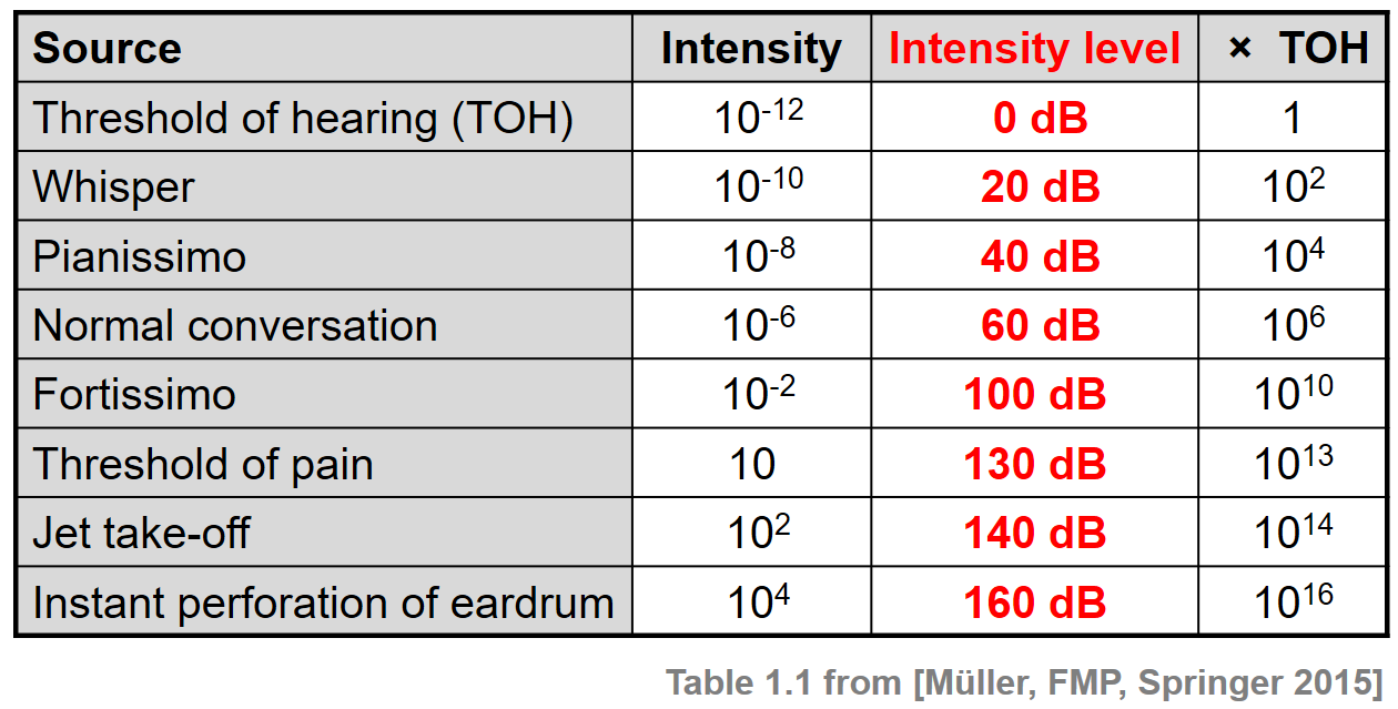
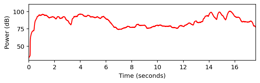
- 예시로 이를 보자.
- 베토벤 5번 교항곡 시작 부분
ipd.Audio("../audio/beeth5_orch_21bars.wav")def compute_power_db(x, Fs, win_len_sec=0.1, power_ref=10**(-12)):
"""Computation of the signal power in dB
Args:
x (np.ndarray): Signal (waveform) to be analyzed
Fs (scalar): Sampling rate
win_len_sec (float): Length (seconds) of the window (Default value = 0.1)
power_ref (float): Reference power level (0 dB) (Default value = 10**(-12))
Returns:
power_db (np.ndarray): Signal power in dB
"""
win_len = round(win_len_sec * Fs)
win = np.ones(win_len) / win_len
power_db = 10 * np.log10(np.convolve(x**2, win, mode='same') / power_ref)
return power_dbFs = 22050
x, Fs = librosa.load("../audio/beeth5_orch_21bars.wav", sr=Fs, mono=True)
win_len_sec = 0.2
power_db = compute_power_db(x, win_len_sec=win_len_sec, Fs=Fs)plot_signal(x, Fs, ylabel='Amplitude', color='gray')
plot_signal(power_db, Fs, ylabel='Power (dB)', color='red')
plt.show()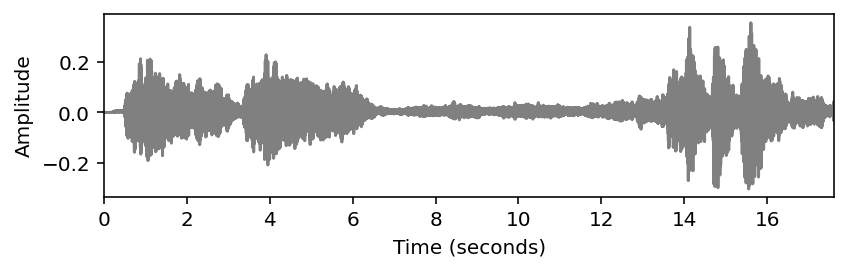
라우드니스(Loudness)
다이나믹과 소리 강도는 소리가 조용한 것에서 큰 것으로 확장되는 규모로 소리를 정렬할 수 있는 라우드니스(loudness)라고 불리는 지각적 특성과 관련이 있다.
라우드니스는 주관적인 측정이며, 이는 개별 청취자(예: 나이는 소리에 대한 인간의 귀의 반응에 영향을 미치는 요인 중 하나)뿐만 아니라 지속 시간(duration) 또는 주파수와 같은 다른 소리 특성에도 영향을 미친다.
- 예를 들어, 사람은 200ms 동안 지속되는 소리가 50ms 동안만 지속되는 유사한 소리보다 더 크게 느껴진다.
- 게다가, 강도는 같지만 주파수가 다른 두 소리는 일반적으로 동일한 라우드니스로 인식되지 않는다.
- 정상적인 청력을 가진 사람은 2~4kHz 정도의 소리에 가장 민감하며, 낮은 주파수뿐만 아니라 높은 주파수에서도 감도가 감소한다.
정신음향(psychoacoustic) 실험을 바탕으로 주파수에 따른 순수 음색의 라우드니스는 단위 폰(unit phon)으로 결정되고 표현되어 왔다.
다음 그림은 동일한 음량 윤곽선(equal loudness contours)을 보여준다. 각 윤곽선은 폰(phon)으로 주어진 고정된 음량에 대해 (로그로 간격을 둔) 주파수 축에 대한 소리 강도를 지정한다. 하나의 폰 단위는 1000Hz의 주파수에 대해 정규화되며, 여기서 하나의 폰 값은 dB 단위의 강도 수준과 같다. 0폰의 윤곽선은 주파수에 따라 청각 임계값(threshold of hearing)이 어떻게 달라지는지를 보여준다.
Image("../img/2.music_representation/FMP_C1_F21.png", width=400)
- 윤곽선은 가중치 함수에 의해 대략적으로 설명될 수 있다. 다음 코드 셀에서 동일한 음량 윤곽선에 질적으로 근사하는 함수의 예를 찾을 수 있다.
def compute_equal_loudness_contour(freq_min=30, freq_max=15000, num_points=100):
"""Computation of the equal loudness contour
Args:
freq_min (float): Lowest frequency to be evaluated (Default value = 30)
freq_max (float): Highest frequency to be evaluated (Default value = 15000)
num_points (int): Number of evaluation points (Default value = 100)
Returns:
equal_loudness_contour (np.ndarray): Equal loudness contour (in dB)
freq_range (np.ndarray): Evaluated frequency points
"""
freq_range = np.logspace(np.log10(freq_min), np.log10(freq_max), num=num_points)
freq = 1000
# Function D from https://bar.wikipedia.org/wiki/Datei:Acoustic_weighting_curves.svg
h_freq = ((1037918.48 - freq**2)**2 + 1080768.16 * freq**2) / ((9837328 - freq**2)**2 + 11723776 * freq**2)
n_freq = (freq / (6.8966888496476 * 10**(-5))) * np.sqrt(h_freq / ((freq**2 + 79919.29) * (freq**2 + 1345600)))
h_freq_range = ((1037918.48 - freq_range**2)**2 + 1080768.16 * freq_range**2) / ((9837328 - freq_range**2)**2
+ 11723776 * freq_range**2)
n_freq_range = (freq_range / (6.8966888496476 * 10**(-5))) * np.sqrt(h_freq_range / ((freq_range**2 + 79919.29) *
(freq_range**2 + 1345600)))
equal_loudness_contour = 20 * np.log10(np.abs(n_freq / n_freq_range))
return equal_loudness_contour, freq_rangeequal_loudness_contour, freq_range = compute_equal_loudness_contour()
plot_signal(equal_loudness_contour, T_coef=freq_range, figsize=(6,3), xlabel='Frequency (Hz)',
ylabel='Intensity (dB)', title='Equal loudness contour', color='red')
plt.xscale('log')
plt.grid()
plt.show()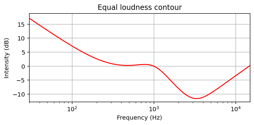
- 동일 힘을 가지는 처프 신호
- 이제 30Hz에서 시작하여 10000Hz로 끝나는, 주파수가 기하급수적으로 증가하는 차프 신호에 대한 작은 실험을 해보자.
- 먼저, 전체 시간 간격에 걸쳐 동일한 강도의 차프 신호를 생성한다. 이 신호를 들을 때는 주파수가 증가함에 따라 신호가 먼저 커지고 약 4000Hz의 주파수를 지나면 다시 부드러워지는 느낌이 든다.
def generate_chirp_exp(dur, freq_start, freq_end, Fs=22050):
"""Generation chirp with exponential frequency increase
Args:
dur (float): Length (seconds) of the signal
freq_start (float): Start frequency of the chirp
freq_end (float): End frequency of the chirp
Fs (scalar): Sampling rate (Default value = 22050)
Returns:
x (np.ndarray): Generated chirp signal
t (np.ndarray): Time axis (in seconds)
freq (np.ndarray): Instant frequency (in Hz)
"""
N = int(dur * Fs)
t = np.arange(N) / Fs
freq = np.exp(np.linspace(np.log(freq_start), np.log(freq_end), N))
phases = np.zeros(N)
for n in range(1, N):
phases[n] = phases[n-1] + 2 * np.pi * freq[n-1] / Fs
x = np.sin(phases)
return x, t, freqFs = 22050
freq_start = 30
freq_end = 10000
dur = 10
x, t, freq = generate_chirp_exp(dur, freq_start, freq_end, Fs=Fs)
fig, ax = plt.subplots(2, 2, gridspec_kw={'width_ratios': [1, 0.05],
'height_ratios': [3, 2]}, figsize=(7, 5))
N, H = 1024, 512
X = librosa.stft(x, n_fft=N, hop_length=H, win_length=N, pad_mode='constant')
plot_matrix(np.log(1+np.abs(X)), Fs=Fs/H, Fs_F=N/Fs, ax=[ax[0,0], ax[0,1]],
title='Spectrogram of chirp', colorbar=True)
win_len_sec = 0.1
power_db = compute_power_db(x, win_len_sec=win_len_sec, Fs=Fs)
plot_signal(power_db, Fs=Fs, ax=ax[1,0], title='Sound power level', ylabel='Power (dB)', color='red')
ax[1,0].set_ylim([103, 137])
ax[1,1].set_axis_off()
plt.tight_layout()
plt.show()
display(Audio(x, rate=Fs) )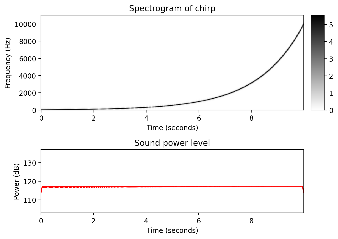
- 동일 라우드니스를 가지는 처프 신호
- 둘째로, 위에서 생성된 동일 라우드니스 윤곽에 따라 신호의 진폭(amplitude)을 조정한다.
- 이 경우 전체 주파수 범위를 통해 스위핑할 때 결과로 발생하는 처프 신호의 라우드니스가 동일한 것으로 보인다.
def generate_chirp_exp_equal_loudness(dur, freq_start, freq_end, Fs=22050):
"""Generation chirp with exponential frequency increase and equal loudness
Args:
dur (float): Length (seconds) of the signal
freq_start (float): Starting frequency of the chirp
freq_end (float): End frequency of the chirp
Fs (scalar): Sampling rate (Default value = 22050)
Returns:
x (np.ndarray): Generated chirp signal
t (np.ndarray): Time axis (in seconds)
freq (np.ndarray): Instant frequency (in Hz)
intensity (np.ndarray): Instant intensity of the signal
"""
N = int(dur * Fs)
t = np.arange(N) / Fs
intensity, freq = compute_equal_loudness_contour(freq_min=freq_start, freq_max=freq_end, num_points=N)
amp = 10**(intensity / 20)
phases = np.zeros(N)
for n in range(1, N):
phases[n] = phases[n-1] + 2 * np.pi * freq[n-1] / Fs
x = amp * np.sin(phases)
return x, t, freq, intensityx_equal_loudness, t, freq, intensity = generate_chirp_exp_equal_loudness(dur, freq_start, freq_end, Fs=Fs)
fig, ax = plt.subplots(2, 2, gridspec_kw={'width_ratios': [1, 0.05],
'height_ratios': [3, 2]}, figsize=(7, 5))
N, H = 1024, 512
X = librosa.stft(x_equal_loudness, n_fft=N, hop_length=H, win_length=N, pad_mode='constant')
plot_matrix(np.log(1+np.abs(X)), Fs=Fs/H, Fs_F=N/Fs, ax=[ax[0,0], ax[0,1]],
title='Spectrogram of chirp with equal loudness', colorbar=True)
win_len_sec = 0.1
power_db = compute_power_db(x_equal_loudness, win_len_sec=win_len_sec, Fs=Fs)
plot_signal(power_db, Fs=Fs, ax=ax[1,0], title='Sound power level', ylabel='Power (dB)', color='red')
ax[1,0].set_ylim([103, 137])
ax[1,1].set_axis_off()
plt.tight_layout()
plt.show()
display( Audio(x_equal_loudness, rate=Fs) )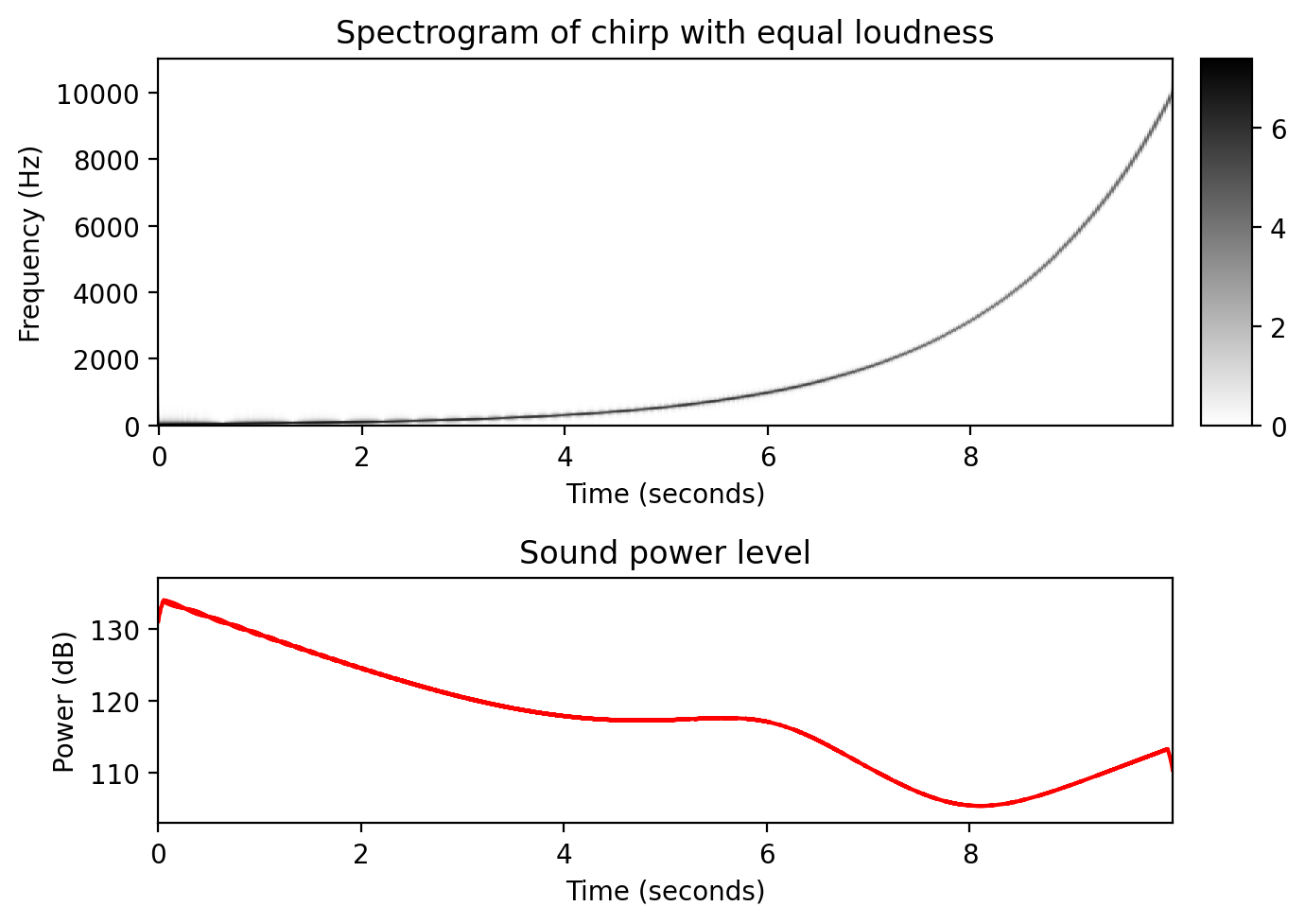
음색 (Timbre)
- 음높이, 음량, 지속 시간 외에도 음색(timbre) 또는 톤 컬러(tone color)라고 하는 사운드의 또 다른 기본적인 측면이 있다.
- 음색을 사용하면 바이올린, 오보에 또는 트럼펫의 음색이 같은 음높이와 같은 크기로 연주되더라도 청취자가 음악적 음색을 구별할 수 있다.
- 음색의 측면은 파악하기가 매우 어렵고 주관적이다.
- 예를 들어, 악기 소리는 밝다, 어둡다, 따뜻하다, 거칠다 등의 단어로 설명될 수 있다.
- 연구원들은 시간 및 스펙트럼 변화, 음조 및 잡음과 같은 구성 요소의 유무 또는 음의 일부 부분에 대한 에너지 분포와 같은 보다 객관적인 소리의 특성과의 상관 관계를 살펴봄으로써 음색에 접근하려고 했다.
엔벨로프와 ADSR 모형(Envelope and ADSR Model)
- 소리의 음색에 영향을 미치는 한 가지 소리 특성은 파형의 엔벨로프(envelope)이며, 이는 진폭에서 극단을 나타내는 매끄러운 곡선으로 간주될 수 있다.
- 음향 합성에서 생성되는 신호의 엔벨로프는 어택(attack, A), 디케이(decay, D), 서스테인(sustain, S), 릴리스(release, R) 단계로 구성된 ADSR이라는 모델에 의해 종종 설명된다.
- 4단계의 상대적 지속 시간과 진폭은 합성된 음색이 어떻게 들릴지에 큰 영향을 미친다.
- 다음 그림은 이상적인 ADSR 모델과 피아노와 바이올린 사운드의 엔벨로프(단음 C4 재생)를 보여준다.
Image("../img/2.music_representation/FMP_C1_F22a-23.png", width=800)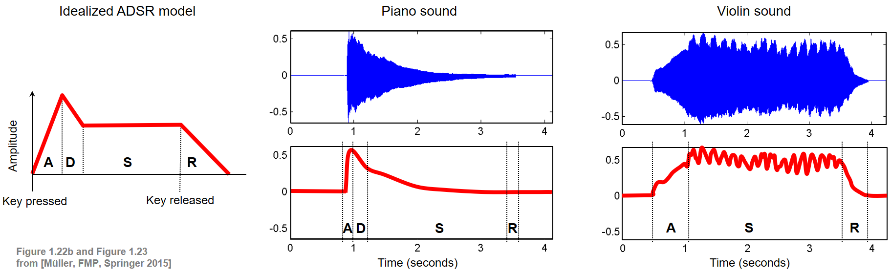
그림에서 알 수 있듯이, 하나의 음을 연주하면 이미 주기적인 요소뿐만 아니라 비주기적인 요소를 포함하여 시간이 지남에 따라 지속적으로 변화할 수 있는 특성을 가진 복잡한 음향 혼합물이 생성된다.
어택(attack) 단계 동안, 소리는 보통 넓은 주파수 범위에 걸쳐 소음 같은 구성 요소로 축적된다. 소리가 시작될 때 소음과 같은 짧은 지속 시간의 소리를 과도음/트랜지언트(transient)라고 한다.
디케이(decay) 단계 동안, 소리는 안정화되고 일정한 주기 패턴에 도달한다.
서스테인(sustain) 단계 동안, 에너지는 꽤 일정하게 유지된다.
릴리스(release) 단계에서는 소리가 사라진다.
다음 코드 셀에서, 이상화된 ADSR 모델을 생성한다.
def compute_adsr(len_A=10, len_D=10, len_S=60, len_R=10, height_A=1.0, height_S=0.5):
"""Computation of idealized ADSR model
Args:
len_A (int): Length (samples) of A phase (Default value = 10)
len_D (int): Length (samples) of D phase (Default value = 10)
len_S (int): Length (samples) of S phase (Default value = 60)
len_R (int): Length (samples) of R phase (Default value = 10)
height_A (float): Height of A phase (Default value = 1.0)
height_S (float): Height of S phase (Default value = 0.5)
Returns:
curve_ADSR (np.ndarray): ADSR model
"""
curve_A = np.arange(len_A) * height_A / len_A
curve_D = height_A - np.arange(len_D) * (height_A - height_S) / len_D
curve_S = np.ones(len_S) * height_S
curve_R = height_S * (1 - np.arange(1, len_R + 1) / len_R)
curve_ADSR = np.concatenate((curve_A, curve_D, curve_S, curve_R))
return curve_ADSRcurve_ADSR = compute_adsr(len_A=10, len_D=10, len_S=60, len_R=10, height_A=1.0, height_S=0.5)
plot_signal(curve_ADSR, figsize=(4,2.5), ylabel='Amplitude', title='ADSR model', color='red')
plt.show()
curve_ADSR = compute_adsr(len_A=20, len_D=2, len_S=60, len_R=1, height_A=2.0, height_S=1.2)
plot_signal(curve_ADSR, figsize=(4,2.5), ylabel='Amplitude', title='ADSR model', color='red')
plt.show()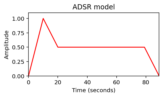

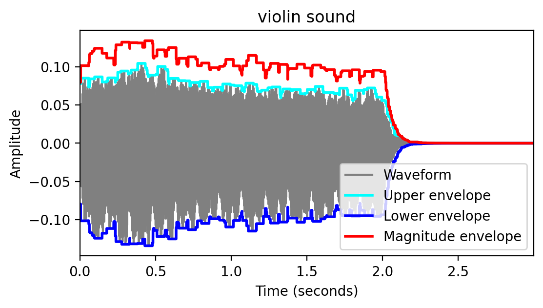
ADSR 모델은 단순화된 형태이며 특정 악기에서 생성되는 톤의 진폭 엔벨로프에 대한 의미 있는 근사치만 산출한다.
예를 들어, 위와 같은 바이올린 소리는 ADSR 모델에 의해 잘 근사되지 않는다.
- 우선 음량을 점차 늘려가며 부드럽게 연주하기 때문에 어택 국면이 퍼진다. 게다가, 디케이 단계가 없는 것처럼 보이고 그 이후의 서스테인 단계는 일정하지 않다; 대신 진폭 엔벨로프는 규칙적인 방식으로 진동한다. 바이올린 연주자가 활로 현을 켜는 것을 멈추면 릴리즈 단계가 시작된다. 그리고 나서 그 소리는 빠르게 사라진다.
엔벨로프 계산
- 파형의 엔벨로프를 계산하는 방법은 여러 가지가 있다. 다음에서는 각 윈도우 섹션에 최대 필터를 적용하여 간단한 슬라이딩 윈도우 방식을 사용한다. 다음 코드 셀에서는 주어진 파형의 상한 엔벨로프와 하한 엔벨로프 및 파형의 크기 엔벨로프를 계산한다.
def compute_envelope(x, win_len_sec=0.01, Fs=4000):
"""Computation of a signal's envelopes
Args:
x (np.ndarray): Signal (waveform) to be analyzed
win_len_sec (float): Length (seconds) of the window (Default value = 0.01)
Fs (scalar): Sampling rate (Default value = 4000)
Returns:
env (np.ndarray): Magnitude envelope
env_upper (np.ndarray): Upper envelope
env_lower (np.ndarray): Lower envelope
"""
win_len_half = round(win_len_sec * Fs * 0.5)
N = x.shape[0]
env = np.zeros(N)
env_upper = np.zeros(N)
env_lower = np.zeros(N)
for i in range(N):
i_start = max(0, i - win_len_half)
i_end = min(N, i + win_len_half)
env[i] = np.amax(np.abs(x)[i_start:i_end])
env_upper[i] = np.amax(x[i_start:i_end])
env_lower[i] = np.amin(x[i_start:i_end])
return env, env_upper, env_lower
def compute_plot_envelope(x, win_len_sec, Fs, figsize=(6, 3), title=''):
"""Computation and subsequent plotting of a signal's envelope
Args:
x (np.ndarray): Signal (waveform) to be analyzed
win_len_sec (float): Length (seconds) of the window
Fs (scalar): Sampling rate
figsize (tuple): Size of the figure (Default value = (6, 3))
title (str): Title of the figure (Default value = '')
Returns:
fig (mpl.figure.Figure): Generated figure
"""
t = np.arange(x.size)/Fs
env, env_upper, env_lower = compute_envelope(x, win_len_sec=win_len_sec, Fs=Fs)
fig = plt.figure(figsize=figsize)
plt.plot(t, x, color='gray', label='Waveform')
plt.plot(t, env_upper, linewidth=2, color='cyan', label='Upper envelope')
plt.plot(t, env_lower, linewidth=2, color='blue', label='Lower envelope')
plt.plot(t, env, linewidth=2, color='red', label='Magnitude envelope')
plt.title(title)
plt.xlabel('Time (seconds)')
plt.ylabel('Amplitude')
plt.xlim([t[0], t[-1]])
#plt.ylim([-0.7, 0.7])
plt.legend(loc='lower right')
plt.show()
ipd.display(ipd.Audio(data=x, rate=Fs))
return figFs = 11025
win_len_sec=0.05
x, Fs = librosa.load("../audio/piano_c4.wav", sr=Fs)
fig = compute_plot_envelope(x, win_len_sec=win_len_sec, Fs=Fs, title='piano sound')
x, Fs = librosa.load("../audio/violin_c4.wav", sr=Fs)
fig = compute_plot_envelope(x, win_len_sec=win_len_sec, Fs=Fs, title='violin sound')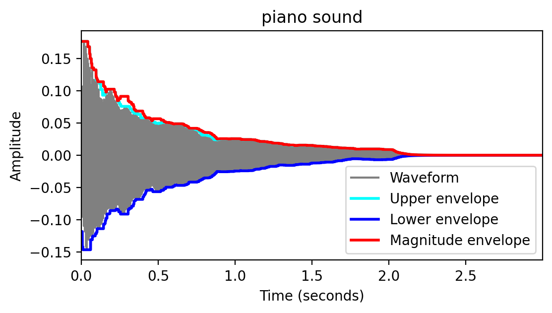
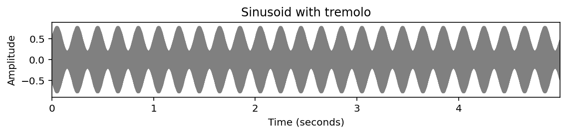
비브라토, 트레몰로 Vibrato and Tremolo
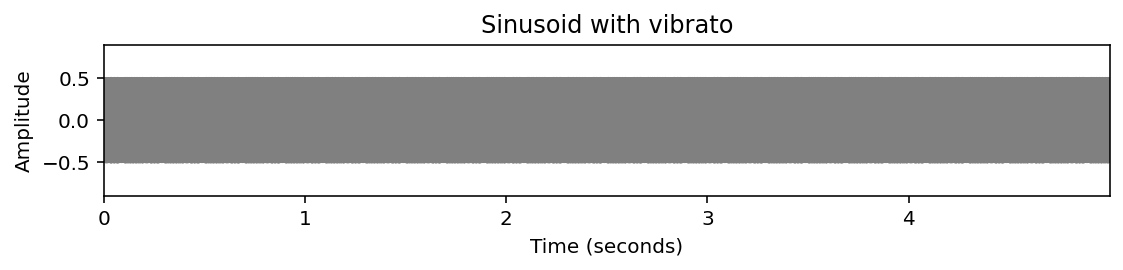
- 바이올린의 예에서 음색과 관련된 다른 현상들이 나타난다. 예를 들어, 진폭의 주기적인 변화를 관찰할 수 있다. 이러한 진폭 변조는 트레몰로(tremolo)로도 알려져 있다.
- 트레몰로의 효과는 진동수의 규칙적인 변화(주파수 변조)로 구성된 음악적 효과인 비브라토와 함께 종종 동반된다.
- 현악 이외에도 비브라토는 인간 가수들이 표현을 더하기 위해 주로 사용된다. 트레몰로와 비브라토가 단순히 강도와 주파수의 국소적인 변화라고 할지라도, 그것들이 반드시 전체적인 음조의 음량이나 음조의 지각된 변화를 불러일으키지는 않는다. 오히려, 그것들은 음악적 음색에 영향을 미치는 특징들이다.
- 다음 코드 셀에서, 단순한 정현파, 비브라토가 있는 정현파, 트레몰로가 있는 정현파를 생성한다.
def generate_sinusoid_vibrato(dur=5, Fs=1000, amp=0.5, freq=440, vib_amp=1, vib_rate=5):
"""Generation of a sinusoid signal with vibrato
Args:
dur (float): Duration (in seconds) (Default value = 5)
Fs (scalar): Sampling rate (Default value = 1000)
amp (float): Amplitude of sinusoid (Default value = 0.5)
freq (float): Frequency (Hz) of sinusoid (Default value = 440)
vib_amp (float): Amplitude (Hz) of the frequency oscillation (Default value = 1)
vib_rate (float): Rate (Hz) of the frequency oscillation (Default value = 5)
Returns:
x (np.ndarray): Generated signal
t (np.ndarray): Time axis (in seconds)
"""
num_samples = int(Fs * dur)
t = np.arange(num_samples) / Fs
freq_vib = freq + vib_amp * np.sin(t * 2 * np.pi * vib_rate)
phase_vib = np.zeros(num_samples)
for i in range(1, num_samples):
phase_vib[i] = phase_vib[i-1] + 2 * np.pi * freq_vib[i-1] / Fs
x = amp * np.sin(phase_vib)
return x, t
def generate_sinusoid_tremolo(dur=5, Fs=1000, amp=0.5, freq=440, trem_amp=0.1, trem_rate=5):
"""Generation of a sinusoid signal with tremolo
Args:
dur (float): Duration (in seconds) (Default value = 5)
Fs (scalar): Sampling rate (Default value = 1000)
amp (float): Amplitude of sinusoid (Default value = 0.5)
freq (float): Frequency (Hz) of sinusoid (Default value = 440)
trem_amp (float): Amplitude of the amplitude oscillation (Default value = 0.1)
trem_rate (float): Rate (Hz) of the amplitude oscillation (Default value = 5)
Returns:
x (np.ndarray): Generated signal
t (np.ndarray): Time axis (in seconds)
"""
num_samples = int(Fs * dur)
t = np.arange(num_samples) / Fs
amps = amp + trem_amp * np.sin(t * 2 * np.pi * trem_rate)
x = amps * np.sin(2*np.pi*(freq*t))
return x, tFs = 4000
dur = 5
freq = 220
amp = 0.5
figsize = (8,2)
x, t = generate_sinusoid(dur=dur, Fs=Fs, amp=amp, freq=freq)
x_vib, t = generate_sinusoid_vibrato(dur=dur, Fs=Fs, amp=amp, freq=freq, vib_amp=6, vib_rate=5)
x_trem, t = generate_sinusoid_tremolo(dur=dur, Fs=Fs, amp=amp, freq=freq, trem_amp=0.3, trem_rate=5)plot_signal(x, Fs=Fs, figsize=figsize, ylabel='Amplitude', title='Sinusoid')
plt.ylim([-0.9, 0.9])
plt.show()
ipd.display(ipd.Audio(data=x, rate=Fs))
plot_signal(x_vib, Fs=Fs, figsize=figsize, ylabel='Amplitude', title='Sinusoid with vibrato')
plt.ylim([-0.9, 0.9])
plt.show()
ipd.display(ipd.Audio(data=x_vib, rate=Fs))
plot_signal(x_trem, Fs=Fs, figsize=figsize, ylabel='Amplitude', title='Sinusoid with tremolo')
plt.ylim([-0.9, 0.9])
plt.show()
ipd.display(ipd.Audio(data=x_trem, rate=Fs))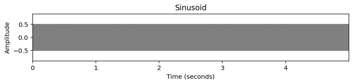
부분음/부분파 (Partials)
아마도 음색을 특징 짓는 가장 중요하고 잘 알려진 속성은 특정 부분파(Partials)의 존재와 그 상대적 강점일 것이다.
부분파는 음악 톤에서 가장 낮은 부분이 기본 주파수(fundamental frequency) 인 지배적 주파수이다.
소리의 부분파는 스펙트로그램으로 시각화된다. 스펙트로그램(spectrogram)은 시간 경과에 따른 주파수 성분의 강도를 보여준다
비조화(inharmonicity)는 가장 가까운 이상고조파(ideal harmonic)에서 벗어나는 부분적 정도를 나타낸다.
명확하게 인식할 수 있는 음정을 가진 음악적 톤과 같은 소리의 경우, 대부분의 부분파는 고조파(harmonics)에 가깝다. 그러나 모든 부분파가 동일한 강도로 발생할 필요는 없다. 다음 그림은 서로 다른 악기에서 재생되는 단일 노트 C4에 대한 스펙트로그램 표현을 보여준다.
Image("../img/2.music_representation/FMP_C1_F23_FourInstruments.png", width=800)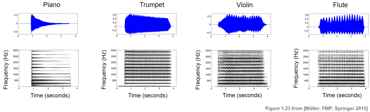
- 음의 기본 주파수(261.6Hz)와 고조파(261.6Hz의 정수 배수) 모두 수평 구조로 보인다.
- 음악 톤의 디케이는 각각의 부분파에서 그에 상응하는 디케이에 의해 반영된다.
- 톤의 에너지의 대부분은 낮은 부분에 포함되어 있고, 높은 부분에 대한 에너지는 낮은 경향이 있다. 이러한 분포는 많은 악기에서 일반적이다. 현악기의 경우, 소리는 풍부한 부분 스펙트럼을 갖는 경향이 있는데, 여기서 많은 에너지가 상부 고조파(harmonics)에도 포함될 수 있다. 이 그림은 또한 트레몰로(특히 플루트의 경우)와 비브라토(특히 바이올린의 경우)를 보여준다.
다른 예
# pure tone
T = 2.0 # seconds
f0 = 1047.0
sr = 22050
t = np.linspace(0, T, int(T*sr), endpoint=False) # time variable
x = 0.1*np.sin(2*np.pi*f0*t)
ipd.Audio(x, rate=sr)X = scipy.fft.fft(x[:4096])
X_mag = np.absolute(X) # spectral magnitude
f = np.linspace(0, sr, 4096) # frequency variable
plt.figure(figsize=(6, 2))
plt.title('pure tone')
plt.plot(f[:2000], X_mag[:2000]) # magnitude spectrum
plt.xlabel('Frequency (Hz)')Text(0.5, 0, 'Frequency (Hz)')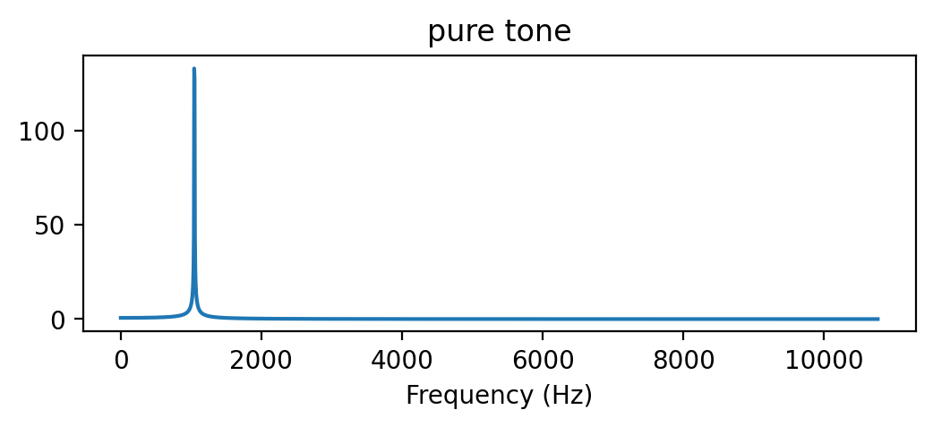
# oboe C6
x, sr = librosa.load('../audio/oboe_c6.wav')
print(x.shape)
ipd.Audio(x, rate=sr)(23625,)X = scipy.fft.fft(x[10000:14096])
X_mag = np.absolute(X)
plt.figure(figsize=(6, 2))
plt.title('oboe C6')
plt.plot(f[:2000], X_mag[:2000]) # magnitude spectrum
plt.xlabel('Frequency (Hz)')Text(0.5, 0, 'Frequency (Hz)')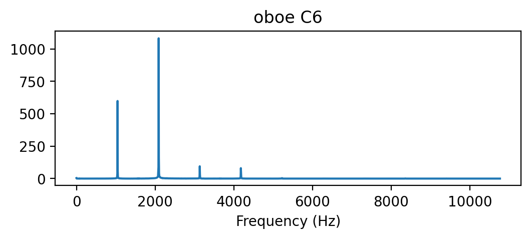
x, sr = librosa.load('../audio/clarinet_c6.wav')
print(x.shape)
ipd.Audio(x, rate=sr)(51386,)X = scipy.fft.fft(x[10000:14096])
X_mag = np.absolute(X)
plt.figure(figsize=(6, 2))
plt.title('clarinet C6')
plt.plot(f[:2000], X_mag[:2000]) # magnitude spectrum
plt.xlabel('Frequency (Hz)')Text(0.5, 0, 'Frequency (Hz)')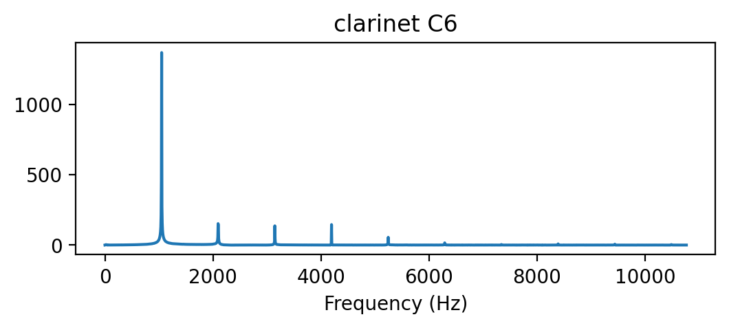
- 부분파의 구성 요소의 상대적 진폭 차이에 주목해보자. 세 신호 모두 거의 동일한 피치와 기본 주파수를 가지고 있지만, 음색은 다르다.
Missing Fundamental
앞서 말했듯이, 소리의 음색은 결정적으로 고조파에 걸친 신호의 에너지 분포에 따라 달라진다. 또한, 인식된 피치의 지각은 기본 주파수뿐만 아니라 더 높은 고조파와 그들의 관계에 따라 달라진다. 예를 들어, 인간은 이 피치와 관련된 기본 주파수가 완전히 누락된 경우에도 톤의 피치를 감지할 수 있다. 이 현상은 “missing fundamental”로 알려져 있다.
다음 코드 예제에서는 음의 중심 주파수(center frequency)의 정수 배수인 주파수를 가진 (가중된) 정현파를 추가하여 소리를 생성한다. 특히 순수 톤(MIDI 피치 𝑝), 고조파가 있는 톤, missing fundamental의 고조파가 있는 톤, 두번 째 순수 톤(MIDI 피치 𝑝+12)을 생성한다.
def generate_tone(p=60, weight_harmonic=np.ones([16, 1]), Fs=11025, dur=2):
"""Generation of a tone with harmonics
Args:
p (float): MIDI pitch of the tone (Default value = 60)
weight_harmonic (np.ndarray): Weights for the different harmonics (Default value = np.ones([16, 1])
Fs (scalar): Sampling frequency (Default value = 11025)
dur (float): Duration (seconds) of the signal (Default value = 2)
Returns:
x (np.ndarray): Generated signal
t (np.ndarray): Time axis (in seconds)
"""
freq = 2 ** ((p - 69) / 12) * 440
num_samples = int(Fs * dur)
t = np.arange(num_samples) / Fs
x = np.zeros(t.shape)
for h, w in enumerate(weight_harmonic):
x = x + w * np.sin(2 * np.pi * freq * (h + 1) * t)
return x, t
def plot_spectrogram(x, Fs=11025, N=4096, H=2048, figsize=(4, 2)):
"""Computation and subsequent plotting of the spectrogram of a signal
Args:
x: Signal (waveform) to be analyzed
Fs: Sampling rate (Default value = 11025)
N: FFT length (Default value = 4096)
H: Hopsize (Default value = 2048)
figsize: Size of the figure (Default value = (4, 2))
"""
N, H = 2048, 1024
X = librosa.stft(x, n_fft=N, hop_length=H, win_length=N, window='hann')
Y = np.abs(X)
plt.figure(figsize=figsize)
librosa.display.specshow(librosa.amplitude_to_db(Y, ref=np.max),
y_axis='linear', x_axis='time', sr=Fs, hop_length=H, cmap='gray_r')
plt.ylim([0, 3000])
# plt.colorbar(format='%+2.0f dB')
plt.xlabel('Time (seconds)')
plt.ylabel('Frequency (Hz)')
plt.tight_layout()
plt.show()Fs = 11025
p = 60
print('Pure tone (p = %s):' % p)
x, t = generate_tone(Fs=Fs, p=p, weight_harmonic=[0.2])
plot_spectrogram(x)
ipd.display(ipd.Audio(data=x, rate=Fs))
print('Tone with harmonics (p = %s):' % p)
x, t = generate_tone(Fs=Fs, p=p, weight_harmonic=[0.2, 0.2, 0.1, 0.1, 0.1, 0.1, 0.1, 0.1, 0.1, 0.1])
plot_spectrogram(x)
ipd.display(ipd.Audio(data=x, rate=Fs))
print('Tone with harmonics and missing fundamental (p = %s):' % p)
x, t = generate_tone(Fs=Fs, p=p, weight_harmonic=[0, 0.2, 0.1, 0.1, 0.1, 0.1, 0.1, 0.1, 0.1, 0.1])
plot_spectrogram(x)
ipd.display(ipd.Audio(data=x, rate=Fs))
print('Pure tone (p = %s):' % (p + 12))
x, t = generate_tone(Fs=Fs, p=p, weight_harmonic=[0, 0.2])
plot_spectrogram(x)
ipd.display(ipd.Audio(data=x, rate=Fs))Pure tone (p = 60):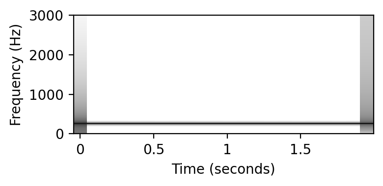
Tone with harmonics (p = 60):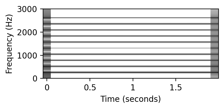
Tone with harmonics and missing fundamental (p = 60):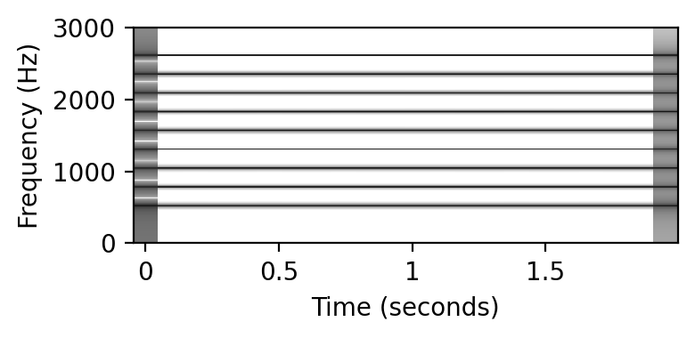
Pure tone (p = 72):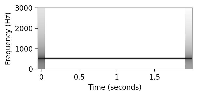
출처:
https://musicinformationretrieval.com/
https://www.audiolabs-erlangen.de/FMP
\(\leftarrow\) 2.2. 기호 표현